Neural Network Compression
Evaluated layer-specific outer product compression to identify structural resilience in deep learning models
The idea
Large fully connected layers are one of the biggest contributors to a neural network's memory footprint, and that footprint becomes a real bottleneck once you're moving parameters between CPU and GPU at scale. For a machine learning course project with three teammates, we wanted to explore one of the simplest possible compression ideas and actually test its limits: what if you replaced a dense weight matrix with the outer product of two vectors?
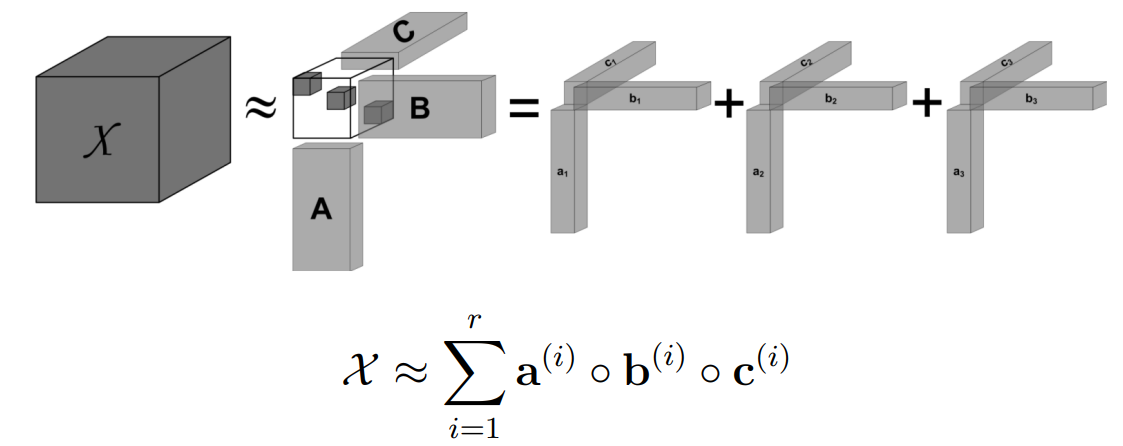
That's an extreme form of low-rank factorization, rank restricted to exactly one, which cuts a layer's parameter count from quadratic (O(nm)) to linear (O(n+m)) in its dimensions. Rather than just implementing it and reporting a single compression number, we wanted to systematically map out where in a network this kind of aggressive compression is viable and where it isn't.
Overview
We built a custom OuterProductLinear layer that replaces a standard nn.Linear layer's weight matrix W ∈ ℝⁿˣᵐ with W = abᵀ, where a ∈ ℝⁿ and b ∈ ℝᵐ are the only learnable parameters. The full weight matrix is reconstructed implicitly during the forward pass, and gradients flow through it via standard backpropagation, so compressed layers train end-to-end with no extra optimization machinery needed.
We applied this to the fully connected layers of a LeNet-5-style CNN trained on Fashion-MNIST, and systematically compressed different layers and layer combinations to isolate:
- Which individual layers tolerate compression (and which collapse)
- How compressing multiple layers together interacts — whether effects are additive, better than additive, or worse
- Whether layer position or layer size is the real driver of compressibility, using two architectures that deliberately isolate one variable from the other
Data
All experiments used Fashion-MNIST, 70,000 single-channel grayscale 28×28 images of clothing items across 10 classes (shirts, shoes, bags, coats, etc.), split into 60,000 training and 10,000 test images, the same split structure as the original MNIST.
Method
We built on a PA3 starting codebase (a LeNet-5 style CNN) and extended it to support compressed linear layers and systematic experimentation across architectures.
Evaluation metrics. We tracked four things for every configuration:
- Classification accuracy on the test set, with drops reported relative to each architecture's uncompressed baseline
- Parameter reduction — percentage decrease in learnable parameters in the fully connected layers vs. baseline
- Training loss — to confirm compressed models actually converged, rather than accuracy differences being an optimization artifact
- Degradation speed — our key normalized metric, defined as:
Degradation Speed = Parameter Reduction (%) / Accuracy Lost (%)
Lower degradation speed is better: it means more memory saved per percentage point of accuracy given up. This let us compare wildly different configurations (a single compressed layer vs. three compressed layers together) on a level footing, rather than just eyeballing raw compression percentages.
Three architectures, each isolating a different variable:
- Test 1 — Unbalanced funnel architecture (FC1: 256→120, FC2: 120→84, FC3: 84→10): the standard CNN pattern where dimensionality shrinks progressively toward the output. This tests compression under realistic, size-mismatched layers.
- Test 2 — Equal-sized layers (FC1 and FC2 both 256→256): deliberately removes the size difference between FC1 and FC2, isolating whether compression tolerance comes from a layer's position in the network or its size.
- Test 3 — Extended middle layers (FC1, FC2, and an added FC2B, all 256→256): tests whether having two middle layers of the same size behave identically, to check if "middle-layer resilience" is a property of position specifically, not a quirk of one particular layer.
Results
Test 1: Unbalanced architecture (baseline: 88% accuracy)
| Configuration | Parameter reduction | Accuracy | Degradation speed |
|---|---|---|---|
| FC1 alone | 72.5% | 74% (−14%) | 0.19 |
| FC2 alone | 23.6% | 80% (−8%) | 0.34 |
| FC3 alone | 1.78% | 74% (−14%) | 7.87 |
| FC1 + FC2 | 96.1% | 74% (−14%) | 0.15 |
| FC2 + FC3 | 25.4% | 60% (−28%) | 1.10 |
| FC1 + FC2 + FC3 | 97.9% | 65% (−23%) | — |
FC1 + FC2 was the standout: compressing both together achieved 96.1% parameter reduction while holding accuracy at 74%, identical to compressing FC1 alone, meaning FC2's compression came essentially "for free" once FC1 was already compressed. FC2 + FC3 was the opposite story: a 28% accuracy loss for only 25.4% parameter reduction, far worse than either layer's individual effect, a clear negative interaction. FC3 alone was catastrophic regardless: minimal compression (1.78%) for a full 14% accuracy hit.
Test 2: Equal-sized layers (baseline: 87% accuracy)
| Configuration | Parameter reduction | Accuracy | Degradation speed |
|---|---|---|---|
| FC1 alone | 48.5% | 75% (−12%) | — |
| FC2 alone | 48.5% | 80% (−7%) | 0.14 |
| FC3 alone | 1.7% | — (−11%) | 6.47 |
| FC1 + FC2 | — | (−22%, worse than additive) | — |
| FC2 + FC3 | 50.2% | (−10%) | 0.20 |
With FC1 and FC2 now the same size, they still lost different amounts of accuracy for identical parameter reduction (48.5%), FC1 dropped 12%, FC2 dropped only 7%. That's the key result of this test: since size was held constant, the difference had to come from position, not size, confirming FC2's resilience isn't just because it's usually smaller in a funnel architecture.
Test 3: Extended middle layers (baseline: 88% accuracy)
| Configuration | Parameter reduction | Accuracy loss | Degradation speed |
|---|---|---|---|
| FC2 alone | 24.7% | 6% | 0.24 |
| FC2B alone | 24.7% | 6% | 0.24 |
| FC1 alone | 24.7% | 14% | 0.57 |
| FC2 + FC2B | 49.4% | 7% | 0.14 (best in this test) |
| FC1 + FC2 + FC2B | 74.1% | 14% | — |
FC2 and FC2B behaved nearly identically when compressed alone, confirming that middle-layer resilience is a property of position, not a quirk specific to one layer. Compressing both middle layers together was the best configuration in this test (0.14 degradation speed), and adding FC1 on top pushed parameter reduction to 74.1% while accuracy loss stayed at 14%, the same loss as compressing FC1 alone, despite compressing roughly three times as much total memory.
Cross-architecture findings
- Middle layers were consistently 1.71–2.4x more compression-resilient than early layers, regardless of architecture or relative layer size, establishing position as the primary driver of compressibility.
- FC3 (the final classification layer) was catastrophic to compress in every architecture we tested (degradation speed 6.47–7.87), despite being the smallest layer, size alone doesn't predict compressibility.
- Interaction effects were highly architecture-dependent and not predictable from single-layer results. The same layer combination (FC2 + FC3) swung from a 28% accuracy loss in Test 1 to just 10% in Test 2, solely due to reconfiguring the surrounding architecture. Combined-layer results deviated 3–8% from what simple addition of individual layer effects would predict.
- Best-performing configurations across all three tests clustered below 0.20 degradation speed — under 0.2% accuracy lost per 1% of memory saved. Worst-performing configurations (anything involving FC3 alone) exceeded 6.0, a 30–50x efficiency gap within the same experiment.
Analysis and discussion
The clearest finding across all three tests: compression effectiveness depends more on a layer's position in the network than its size. Middle layers consistently carry redundant intermediate representations that can absorb aggressive rank-one compression with minimal accuracy cost, while early layers (doing feature extraction) and especially final classification layers are much more sensitive, likely because the final layer directly encodes the decision boundary between classes and has little redundancy to spare.
The interaction effects were the most interesting and least predictable part of the results. Layer combinations didn't behave as the sum of their individual effects, sometimes better (FC1 + FC2 in Test 1), sometimes worse (FC1 + FC2 in Test 2, FC2 + FC3 in Test 1), and which direction it went depended entirely on the surrounding architecture. That's a meaningful finding in its own right: you can't reliably predict a multi-layer compression strategy by testing layers independently and adding up the damage, each architecture needs to be evaluated directly.
Limitations
Our rank-one factorization is intentionally the simplest possible case of low-rank approximation; more expressive approaches (higher-rank factorization, pruning, quantization) likely achieve better accuracy-compression tradeoffs but were outside this project's scope, we wanted to isolate the effect of the most aggressive compression, not find the best one. The network itself is also small: absolute memory savings here are modest compared to what the same technique would yield on a large-scale model, so we couldn't directly validate real-world benefits like reduced memory bandwidth or faster CPU-GPU data transfer. Finally, all models were trained from scratch under the same fixed optimization procedure; techniques like fine-tuning after compression, adaptive learning rates, or extra regularization might meaningfully improve heavily compressed configurations, but we didn't explore them here.
What's next
- Testing higher-rank (rather than strictly rank-one) factorizations to see where the accuracy-compression curve actually bends
- Applying fine-tuning after compression instead of training compressed layers from scratch alongside everything else
- Scaling the approach to a larger network where the absolute memory savings would actually matter in practice
- Combining outer-product compression with pruning or quantization to see whether the position-dependent redundancy we found here compounds with other compression strategies